[Work Log] Work Log
Spent morning considering covariance over loopy graphs. Implemented and example of "shortest geodesic distance", modified to be minimum sum of squared distances between junctions over all paths. This is a generalization of our metric over tree-structured graphs. As anticipated, with loopy graphs, this results in non-positive-definite covariance matrices.
Consider this example, with two paths between nodes (1) and (4), one twice as long as the other.
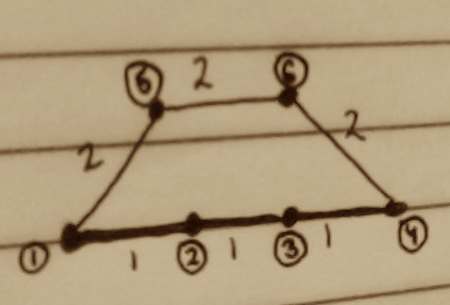
The shortest squared-distance matrix is
 0     1     4     9     4    13
 1     0     1     4     5     8
 4     1     0     1     8     5
 9     4     1     0    13     4
 4     5     8    13     0     4
13     8     5     4     4     0
The code for this is:
d1 = 0:3; % route 1 distances
d2 = 0:2:6; % route 2 distances
D1 = pdist2(d1', d1', 'euclidean').^2;
D2 = pdist2(d2', d2', 'euclidean').^2;
G  = sparse(size(D));
% top-left block is simply a straight path
G(1:length(d1),1:length(d1)) = D1;
% for bottom-left, compute shortest path between nodes through
% junctions
for i = 1:(length(d2)-2)
  i_ = length(d1)+i;
  for j = 1:length(D)
    j_ = j;
    if i_ == j_, G(i_,j_) = 0; G(j_,i_) = 0; continue, end
    G2 = sparse(4,4);
    G2(1,2) = D(i_, 1);
    G2(1,3) = D(i_, length(d1));
    G2(2,3) = D(1,length(d1));
    G2(1,4) = D(i_, j_);
    G2(2,4) = D(1,j_);
    G2(3,4) = D(length(d1),j_);
    d = graphshortestpath(G2', 1,4, 'directed', false);
    G(i_, j_) = d;
    G(j_, i_) = d;
  end
end
At large enough scales, the squared-exponential covariance matrix has negative eigenvalues:
scale = 10;
min(eig(exp(-full(G)/(scale^2*2))))

    ans =

       -0.0134
Thus, this covariance function is not positive definite.
A loopy graph strategy
We need to be able to embed the graph into a Euclidean space that preserves most of the interesting properties.
Here's a simple approach: construct a graph with junctions as vertices and geodesic distance as edge weight. Find the graph's minimum spanning tree, and transform the tree into curve-tree coordinates. For unclaimed curve segments, linearly interpolate between the coordinates of the endpoints.
This is nice, but if an unclaimed curve segment's length is perticularly long, it should act differently than a short (straight) line between the points. To handle this, we introduce a new dimension for each unclaimed curve segment, and allow the transformed segment to have longer length by dipping into this dimension to some extent (with a limit of none for straight lines).
Ideally, all pairs of points on the transformed segment will have the same distance as their geodesic distance in untransformed space. However, this is not possible, because it would contradict the fact that the endpoint distance is defined by the graph distance in the minimum spanning tree. At least we can try to preserve local distances, and a parabolic arc is a reasonable choice for this. How to derive a parabola equation of an appropriate length?
Given the distance between the end-points and the length of the desired curve, we seek a symmetric parabola with an appropriate arc length. Given arc length and end-points, we can compute the focus the parabola (f), and from that we can compute the parabolic equation y = x2/(4f).
Training foreground likelihood
First, reproject curve into second image.
Draw as medial axis w/ width.
Compute inverse medial axis.
Grab all foreground/background pixels in probability map.
create histogram. Try smoothing and/or annealing.
Done.
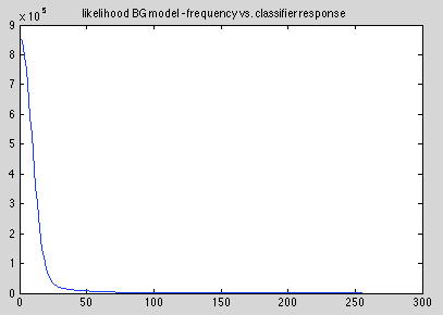
Foreground model:
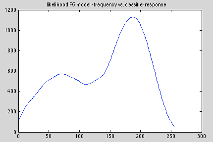
Background model: