
[Work Log] Fire: 10 inference experiments
Ran 10,000 iterations, keeping observation model fixed.
Update: The three plots below are incorrect. corrected plot follows.
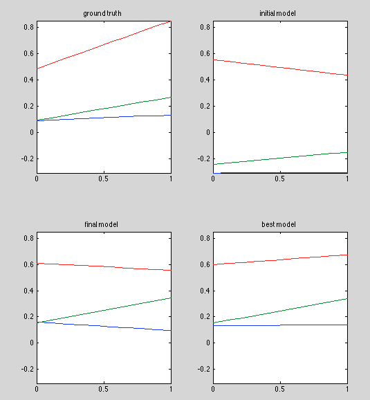
Ground truth model:
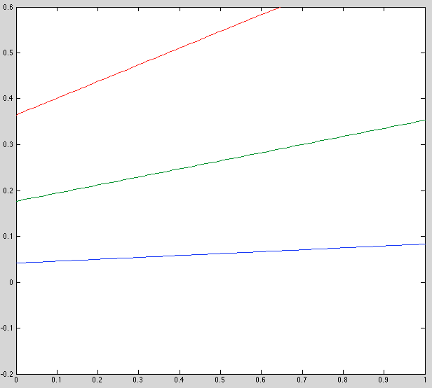
Initial model:
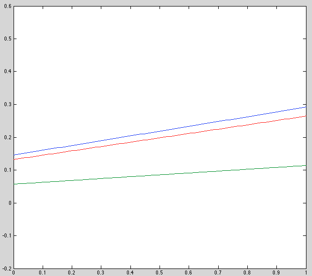
Final model:
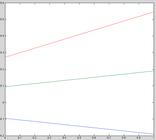
Update: There was a bug in my plotting code for the plots above. Here is the corrected plot, which is more sensible:
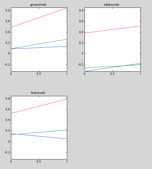
Observations:
- Initial estimate is bad, esp y-offset. Should review this code.
- Recovered results are noticably better. Not perfect, but this may be because we're seeing the final model, not the best one.
- Keeping observation model fixed seems to improve speed by two orders of magnitude (why???)
Run 2: Keep best model
Added a 'best_sample_recorder' to keep track of the best model we've seen.
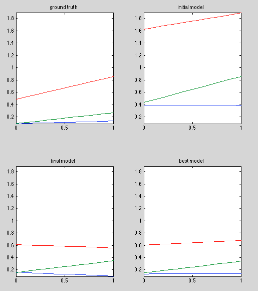
Results
Observations
- Best model is pretty good
- Why is initial model so different from that in the previous run? same model, same random seed.
- Keep in mind, on average only 1/3 of the [0,1] domain is represented in the dataset, because it's divided into "before", "during" and "after" regions.
Discussion
Initial model uses a different observation model, so it's hard to say whether it's good or not. I get the feeling that there's a lot of slack in this model, meaning several different combinations of observed and latent parameters can give nearly equal results.
Also, initial model estimation doesn't correctly handle x-offsets for "during" and "after" regions. TODO: fix this.
Note that the noise epsilon is very large relative to the model's dynamic range. It's hard to visualize, since the plots above are sent through an observation model before noise is added. But the observation model's scaling is around 0.5.
Variability in the latent variable is around 0.3. Observation model scales that to 0.15, then adds noise on the order of 1.0. So signal-to-noise ratio is around 0.15 -- not great. Luckilly we have lots of observations (150 people x 9 time points x 7 observed dimensions), but in our non-synthetic model, I hope our noise is smaller.
Run 3: Improved initial model estimate
SVN REVISION: 16742
Description: Fixed initial model estimate by centering each region at x=0. See model.cpp:partition_observations().
# iterations: 10,000 iterations
Running time: 0:18.53
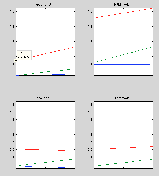
Results:

Summary:
Initial model has changed, but initial offset is still way off. Other models (final and best) are the same.
Discussion:
Need to dig more into the initial estimation code. Is boost's RNG seeded with current time?
Run 4: fixed observation parameters
SVN REVISION: 16743
Goal: See if fixing observation parameters (A, B) improve line-fits. If so, issue is in observation parameters. If not, issue is with line-fitting.
Running time: 0:18.26
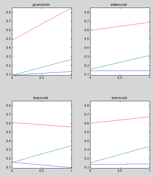
Results:
Discussion:
Bad results; issue is probably in line-fitting, not estimation of observation model.
Run 5: fixed observation parameters (take 2)
Description: Found a bug when using fixed offset B -- wasn't subtracting offset before doing PCA to find A.
Revision: 16744
Results:
Discussion: No change. In retrospect, this change only applies when not using fixed observation parameters, so no change is to be expected. But a good bug to fix for later on!
Run 6:
Description:
Found another bug: when projecting points onto pincipal component, if the direction vector \(d\) isn't normalized to 1, the projected points are off by a factor of \(|d|^2\). The observation equation is given by:
Revision: 16745
Invocation:
# On bayes01
cd ~ksimek/src/fire/src/piecewise_linear/test
./test_inference > /dev/null
cat results.txt | \
    awk '{row=NR%7; if(row == 3 || row == 4) print;}' \
    > ~/tmp/lin.txt

# on local machine
rsync -avz v01:tmp/lin*.txt ~/tmp/

# in matlab on local machine
cd ~ksimek/work/src/fire/src/matlab/in_progress
figure
lin = load('~/tmp/lin7_1.txt')'
lin3 = reshape(lin, [3, 2, 4])
visualize_pl_result(lin3, ...
    {'ground truth', ...
    'initial model', ...
    'final model', ...
    'best model'})
Results:
Discussion:
Finally getting good initial estimates. In fact, initial estimate is the optimal estimate when A and B are known. The best model doesn't look perfect, especially in the red curve, but there seems to be significant variance in the red curve estimator, as shorn in "final model".
Run 7: Initial estimate of A
Description: Time to add initial estimation of A. Sampling will still only estimate latent parameters. I'm curious how close this will be to optimal. I'm forcing the ground-truth A to have unit-length so the experimental results are comparable to the ground truth.
Invocation: see previous
Revision: 16746
Baseline: The results below are estimates of the linear model when A is known.

Results: Below are results of sampling, using an estimate of A from the noisy data

Discussion:
Initial estimate is slightly worse in the green and blue curves, but still in the ballpark, as we would hope. As observation noise decreases, this estimate should improve.
It's notable that HMC still can't find a better model. This is good news for the quality of our estimate.
Run 8: initial estimate of A and B
Description: Adding initial estimation of B to the test.
Invocation: see previous
Results:

Discussion:
Much worse. This could be caused by overestimating the magitude of (B), while understimating the magnitude of (b) (which can result in identical models due to our model being overdefined). Since (b) currently adds positive offset to all observations, estimating (B) as the mean over observations could is likely to capture some of (b).
Probably the best way to evaluate is to measure prediction error.
Update run 9 shows that this model predicts quite well, despite having different model parameters.
Discussion - Scaling and offset
I'm starting to think we should consider preprocessing the immunity data bafore passing it through this model, for two reasons
1. poorly scaled data; correlated noise
It seems too easy that we can solve for 'A' using simple PCA. Said differently, dynamics are the interesting part of our model, but A is determined irrespective of dynamics.
The observation transformation A has an intuitive interpretation as the direction of greatest variation in the data, after taking dynamics into account. The problem with this is that if data is badly scaled, the direction of greatest variation will come from the noise, not the dynamics. If possible, we’d prefer to separate variation due to noise from variation due to dynamics. That way, A can capture the dynamic relationships between variables (e.g. IL-6 and IL-5 both start low and end high), not just correlation (IL-6 and IL-5 co-vary, but no temporal information).
For this reason, it might help to "whiten" the data by PCA, so the inferred direction of A is more likely to capture dynamics only.
2. Variability in immunity measurements
Second, I’ve been thinking on the fact that individuals’ immunity values differ significantly in scale and offset. From what I understand, much of this variation occurs within “plate”, i.e. its a byproduct of laboratory conditions, not immunity dynamics. This could affect our clustering, as the latent slope and y-intercept parameters depend directly on the data’s scale and offset. As a result, I fear our learned clusters will reflect different groups of “laboratory conditions”, rather than different groups of immunity dynamics.
We could replace readings with z-score within each person, but this has two problems:
- readings that are relatively constant but legitimately high would seem more typical than they are.
- extremely steep changes over time would tend to flatten. similarly, relatively low slopes would tend to look higher after transforming.
No obvious answer; may need to try several solutions.
Run 9: Held-out error
Description: Since our model is overdefined, comparing model parameters is no longer a good indicator of model quality. Instead, we should held-out data to evaluate the predictive power of the model
Method: hold out 20% of data, measure log-likelihood for (a) ground truth model, (b) initial model estimate. Two cases: 1. using global mean for B, PCA for A, 2. using ground truth A and B.
Results:
Training error:
------------

    Ground truth:              -13301.3
    Ana. Soln (Known A, B):    -13295.2
    Ana. Soln (Inferred A, B): -13318.3

Testing error:
-----------

    Ground Truth:               -1886.17
    Ana. Soln (Known A, B):     -1887.3
    Ana. Soln (Inferred A, B):  -1887.06
Discussion:
Training error is better for analytical solution with known A and B, which what we'd expect if the analytical solution was the true optimum. When A and B are inferred, training error is worse, since PCA doesn't account for dynamics.
Prediction error is worse than ground truth for all models, which is a good sanity check. But they're all in a very tight ballpark (less than 1.0), which suggests that we aren't overfitting. A better test would be to compare against one or more simpler models, but these results are good enough to proceed.
One good conclusion is that even though inferring A and B results in vastly different latent models (see run #8), the prediction is just as good.
Run 10: Whitening before inference
Description: transforming observations so they follow a standard m.v. Gaussian may help in infering. Test prediction error and compare against run #9 errors (should be nearly identical). Revision: 16756
Method: transform data by PCA. Using linear regression to infer initial direction (since PCA is out). Force B to be zero. Fit model. Evaluate held-out error after transforming back to data space.
Results:
("Error" is average negative log likelihood over 150 points)

Ground truth
------------
    Training error: 88.6756
    Prediction error: 90.3623

Estimated Model
--------------
    Raw data; A,B from PCA
    ---------
    Training error: 88.7887
    Prediction error: 90.5986

    Raw data; A,B from Regression
    ------------
    Training error: 88.6285
    Prediction error: 90.4405

    Whiteened Data; A,B from Regression
    --------------
    Training error: 93.8502
    Prediction error: 95.7252
Discussion:
Training and prediction error is worse for whitened data, which is contrary to my expectation. In retrospect, we're fitting to different data, so it's not too surprising that it predicts worse. The story may be different if the data is truely poorly scaled. Our example data was already well scaled, so its not a great test.
But in the end, its defnitely clear that whitening isn't innocuous, and possibly harmful.
Mid-term TODO
- Tuning HMC
- refactor model
- Start and end times out of model
- epsilon per-dimension
- missing data
- Add offset constraints (continuous model)
- clustering
Meta-notes on experiments
- always test on synthetic data first
- always test on a simpler model first (fix some parameters)
- always have a visualization in mind when running a test.